How to Clean Text Data in Excel: A Beginner’s Guide 

Introduction 

Clean text data in Excel is essential for accurate, reliable analysis.When working with text data on Excel, dirty data can result in misleading insights, poor decision making, which can lead to revenue loss. With the right tools and techniques, you can clean text data in Excel quickly and confidently, even as a beginner. 

As a data analyst, you don’t always have control over the quality of the data you receive. The good news is that Excel has a wide range of functions, formulars and processes, to help transform your data from dirty to clean.  

In this article, you’ll learn techniques to clean text data efficiently in Excel. Whether you’re dealing with duplicate data, extra space, unwanted characters or inconsistent format, this step-by-step guide will equip you with the skills to ensure your data is accurate, consistent and ready for analysis. 

Prerequisites 

Before cleaning text data in Excel, create a backup of your dataset so you can easily restore it if needed. To effectively follow along with this guide and get the most out of it, it is essential that you: 

• Have a basic understanding of Excel including formulas and functions 

• Have Microsoft Excel installed on your computer. 

• Download the dataset to follow along. 

Step-by-Step Guide to Clean Text Data in Excel 

Getting Started with Text Cleaning in Excel

Excel provides a variety of tools to clean and organize your text data, making it ready for analysis.

In this guide, we’ll walk through some of the most effective ways data analysts clean text data in Excel, using a messy retail dataset to demonstrate key procedures, including how to:

• Remove duplicates 

• Handle blank cells 

• Remove unwanted characters 

• Trim Leading and Lagging Spaces 

• Change text case 

• Replacing Multiple Characters 

• Split delimited text 

• Reverse text characters 

In this guide, we’ll explore a retail transactions dataset that contains various fields relating to customer purchase, such as Transaction ID, Transaction Date, Customer Email, Quantity Sold, and more.

For this guide we will only be focusing on the text data contained in the dataset. You can download the dataset to follow along using this link: Dataset 

Before you start making changes, create a copy of the raw data. This way, if something goes wrong or important information is accidentally removed, you’ll have the original to fall back on.

Our focus will be on the text-based fields, such as“Transaction ID”, “Customer Name”, “Customer Email”, “Location”, “Product Name”, “Category”, “Payment Method” and “Sales Representatives”. 

After you’ve created a copy of the raw data, go through the dataset and delete the columns that are unnecessary for your guide, which are the non-text columns on the dataset. 

You can remove other columns like “Transaction Date”, “Quantity Sold”, and “Discount Applied” to clean up your view. 

Remove Duplicates 

Duplicate values in a dataset are records that show up more than once. This can lead to skewed analysis, inflated predictions, and inaccurate conclusions. Removing duplicate rows is a core part of how you clean text data in Excel, especially in datasets prone to repetition. It helps maintain data integrity, data quality, and ensures data uniqueness. 

Excel provides built-in tools to quickly identify and eliminate duplicate entries, allowing you to clean your data in just a few steps. 

If we consider a sample retail dataset that contains duplicate rows, to remove the duplicate values you: 

1. In the menu bar, select the Data tab, then under Data Tools, select Remove Duplicates 

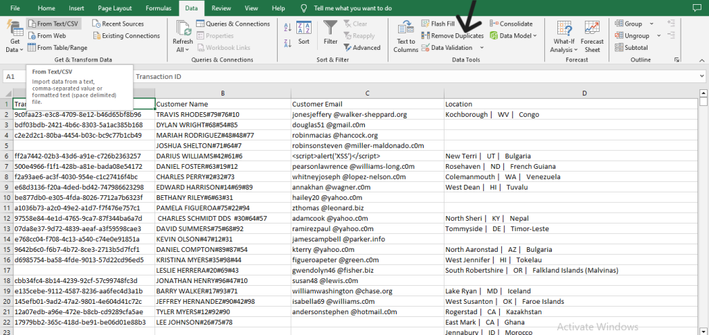
Removing duplicate rows in excel 

2. Ensure that the box next to My Data Has Headers is checked then click on Select All to select all the columns, if not already selected. Finally select Ok to carry out the action. 

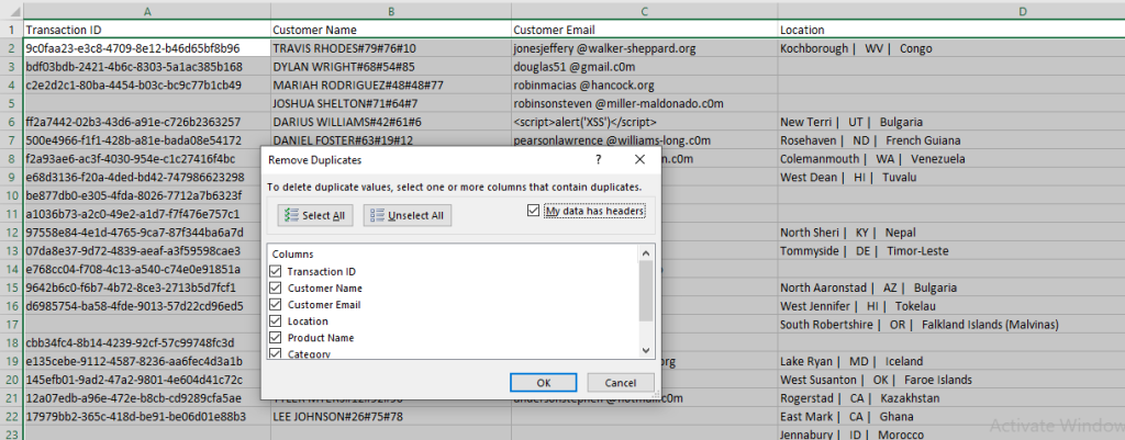
Selecting column to check for duplicates 

3. After you complete the operation, Excel displays a pop-up box showing how many duplicate values it removed. Click on ok to remove the pop-up box. 

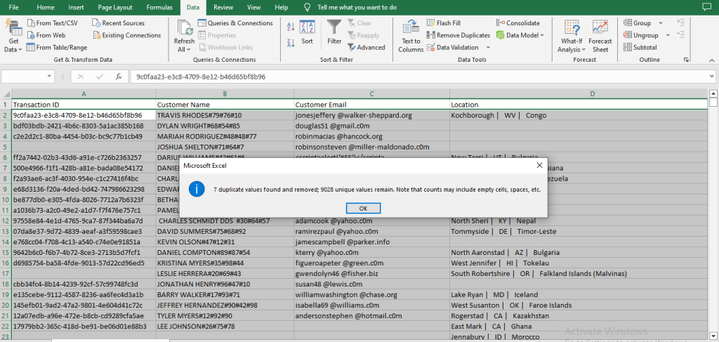
And just like that, with just a few clicks of the mouse we’ve successfully removed all duplicates from the data. 

Handle Blank Cells 

Blank cells indicate missing data which can result from improper data collection, incorrect entries or incomplete records. If left unaddressed, they can lead to a decrease in productivity and inaccurate insights. 

There are multiple ways to handle blanks in Excel depending on the context. 

• Reaching out to the data source, if possible, is one of the best practices for handling missing data, especially when the missing data is crucial for analysis. They may be able to provide the missing data or explain why it wasn’t there in the first place. 

• When working with numerical data, using the average or the median of the available data could serve as an appropriate way to fill the blanks. This needs to be consistent with the business rules. 

• Deleting the rows with blank data would be appropriate if only a few rows are missing data and/or the data is not critical for your analysis. 

• Replacing the blank cells with an appropriate placeholder like “Unavailable” ensures clarity without introducing misleading information.This approach is especially helpful when working with text data, as it maintains a consistent structure—crucial when the original data can’t be retrieved. Using ‘Unavailable’ as a placeholder works well because it clearly signals that a value was expected but not captured, without distorting the dataset’s meaning. Since we are working with text data, and we are unable to reach out to the source of the data, this is the method we will use in this guide.  

To select the blank cells and fill them up with a placeholder of our choice, you: 

1. Highlight the necessary columns. Since the dataset we’re working with is only text, we can just go ahead and select the entire dataset. To do this, click on the first column (column A), hold the Shift key and at the same time use your mouse to click on the last column (column I) on the dataset. 

2. After highlighting the entire dataset, hold down the Ctrl key and press G on your keyboard. This opens the Go To dialog box, from which you can highlight only the cells with blanks. 

“Go To” dialog box

3. Next click on Special, which opens a new dialog box with multiple options. Select Blank then click on Ok. This highlights all the blank cells on the dataset. 

Excel “Go To Special” dialog box 

4. After highlighting all blank cells, type a suitable placeholder like “Unavailable.” Rather than pressing Enter, hold down the Ctrl key and press Enter. That keyboard shortcut fills all selected blank cells at once.

Excel spreadsheet with ”Unavailable” filling all blank cells 

That fills all the empty cells with an appropriate placeholder.

Remove Unwanted Characters 

Text data sometimes contain unwanted characters such as extra space, special symbol, or non-printable characters. If not checked, they can affect sorting, filtering and overall data accuracy. 

Excel offers multiple ways to address this issue, but in this guide, we’re going to be focusing on using a combination of the LEFT, FIND and IFERROR functions to remove unwanted characters. To effectively use this combination of functions to remove unwanted characters, you: 

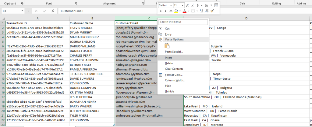
1. Create a new column next to the column you are trying to clean up and give it the same name as the original. To do this you right click the column next to the target column, then select Insert. Since you are attempting to make the changes to column B, right click on column C and select Insert. 

Excel right click menu showing ”Insert” 

2. In the second cell (C2) of the newly created column, write the formula =IFERROR(LEFT(B2, FIND("#", B2, 1) -1), B2). This formula extracts the customer name from column B by selecting only the characters before the first # symbol. It works like this: 

1. FIND(“#”, B2, 1) 

• Locates the position of the first # in cell B2 

• In cell B2, TRAVIS RHODES#79#76#10, the first # is the 14^th character. So the formula FIND("#", B2, 1) returns 14. 

2. LEFT(B2, FIND(“#”, B2, 1) -1) 

• LEFT extracts a specific number of characters from the beginning of the text. 

• So it becomes LEFT(B2, 14 - 1). Which becomes LEFT(B2, 13). Where 13 is the exact number of characters we wish to extract from the text. 

• In cell B2 TRAVIS RHODES#79#76#10 becomes just TRAVIS RHODES. 

3. IFERROR(…., B2) 

• This part of the formula is a safety net.  

• If no ‘#’ is found and an error occurs, then the formula will return to the original B2 value instead.

3. Finally, click on cell C2 and hover your mouse to the fill handle (the bottom right corner of the cell), till your mouse appears as a small black cross. Then double click it to fill the rest of the column. 

“Customer Name” next to the clean version

4. Copy column C, then right click and select Paste Values, before deleting the original “Customer Name” column. Note that you must do this after any data cleaning involving formulas or functions 

And with that you have successfully extracted all the clean customer names by removing all the unnecessary characters. 

Trim Extra Space 

Extra space in text data can lead to inconsistencies, making it difficult to search, sort, or compare values accurately. An effective way to resolve this is to use the TRIM function. This removes trailing, leading and repeated spaces in text data. To use the TRIM function, you: 

1. Start off by creating a new column next to the column you are trying to clean and give it the same name as the original. In this case, create a new column at column C. 

2. In the second cell of the new column (C2), enter =TRIM(B2). This removes any unnecessary space in the text. 

3. Populate the rest of the column by double clicking the fill handle. 

You’ve successfully removed all trailing, leading, and repeated spaces from the column.

Change Text Case 

Inconsistent text capitalization can make your data look unprofessional and harder to analyze. Standardizing text case improves readability and ensures uniformity across your dataset. 

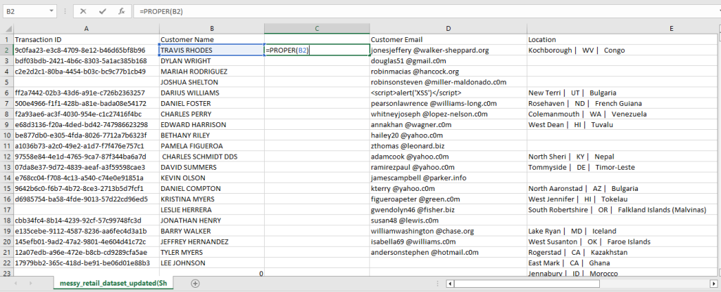
Considering the “Customer Name” column in our dataset, consistency is key. Havin all the names in upper case can feel harsh and harder to scan, especially in long lists. Using the function LOWER to convert the text to lower case makes the text look casual and unprofessional. That is why we will use the PROPER function to convert those text to a proper case (only first letters in upper case), because it gives the text a more professional and polished look, makes it easier on the eyes, and enhances data uniformity. To use the PROPER function, you: 

1. Create a new column next to the column of interest and give it the same name. Here the new column would be column C. 

2. In the second cell of the new column (C2), enter the formula =PROPER(B2). This converts the text from upper case to proper case. 

3. Populate the rest of the cells in the new column. 

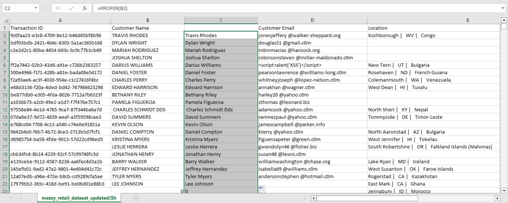
You’ve successfully converted the uppercase text to proper case.

Replacing Multiple Characters 

When you clean text data in Excel, you might encounter multiple unwanted characters such as symbols, punctuation marks or typos. These can cause inconsistencies in your data and interfere with your analysis. 

While Excel doesn’t offer a built-in feature to replace multiple characters at once, you can do it by nesting several SUBSTITUTE functions together.. Along with the SUBSTITUTE function, we will also use the TRIM as well as the PROPER function to clean the entire column in a single go. To do this we: 

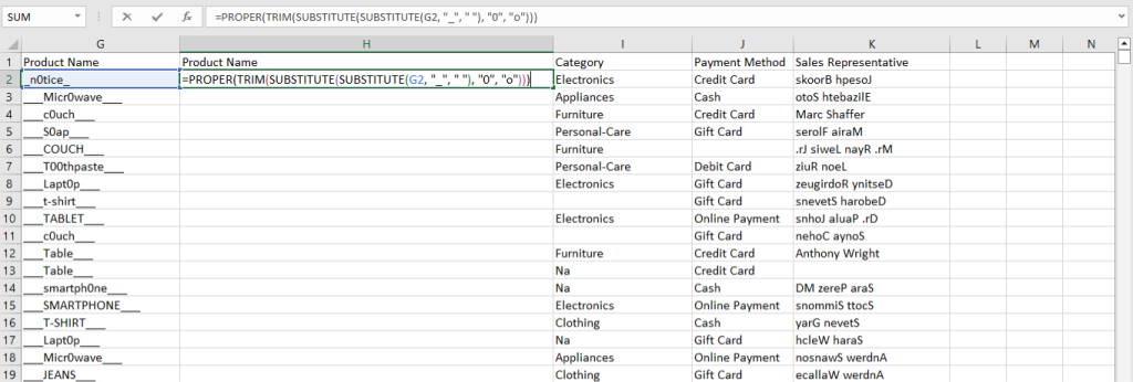
1. As with previous steps, create a new column next to the one you want to clean and name it the same as the original. In this case, we’re cleaning the ‘Product Name’ column. So, the new column would be column H. 

2. In cell H2, write the formula =PROPER(TRIM(SUBSTITUTE(SUBSTITUTE(G2, "_", " "), "0", "o"))). This replaces underscores with space, “0” with “o”, removes any trailing or leading space and converts the text to a proper case.  The formula works this way: 

1. SUBSTITUTE(G2, “_”, ” “) 

• This replaces any underscore “_” with a space “ “. 

2. SUBSTITUTE(……., “0”, “o”) 

• Next, this formula replaces all zero “0” with a lower case “o” 3
• ;p;p
• p

3. TRIM(….)  

• This removes any extra space from the beginning, end, or between words (double spaces). 

4. PROPER(….) 

• Finally, this converts the text to proper case. 

3. Next, auto fill the rest of the cells in the column. 

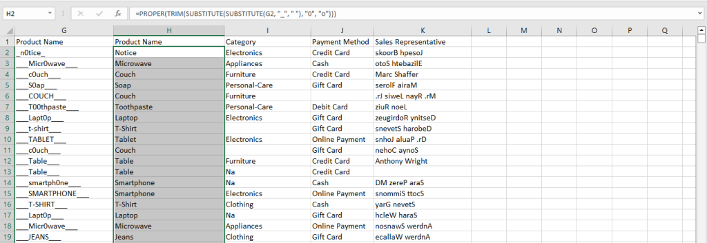
4. The final step is to copy and paste as plain text, before deleting the original “Product Name” column. 

Split Delimited Text 

Sometimes, data can be stored in a single column but contain multiple pieces of information separated by delimiters such as comma, hyphen, or space.

Splitting the delimited text into separate columns makes it easier to analyze specific parts of the data efficiently. 

Excel’s Text to Column feature is straight forward but extremely useful for splitting delimited text. To do this you: 

1. Before using the Text to Column feature, ensure you create enough new columns next to the column you are trying to split, to accommodate the data that will be split. For our data set, that would be two new columns. 

2. Select the column you wish to split. 

3. In the menu bar, select the Data tab, then under Data Tools, select Text to Column. 

4. In the dialog box that appears, select Delimiter, then click on Next. Excel “Convert Text to Columns Wizard 1 

5. In the next dialog box, select Other and input the delimiter you wish to split the column on. In this case, we are splitting the column on the | character as the delimiter, then click Next. 

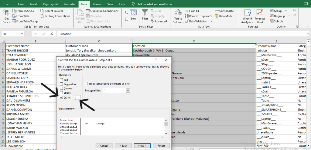
Excel “Convert Text to Columns Wizard 2 

6. Since the column we are working on is text data, select the Text as the Column Data Format on the next dialog box. Then click on Finish. 

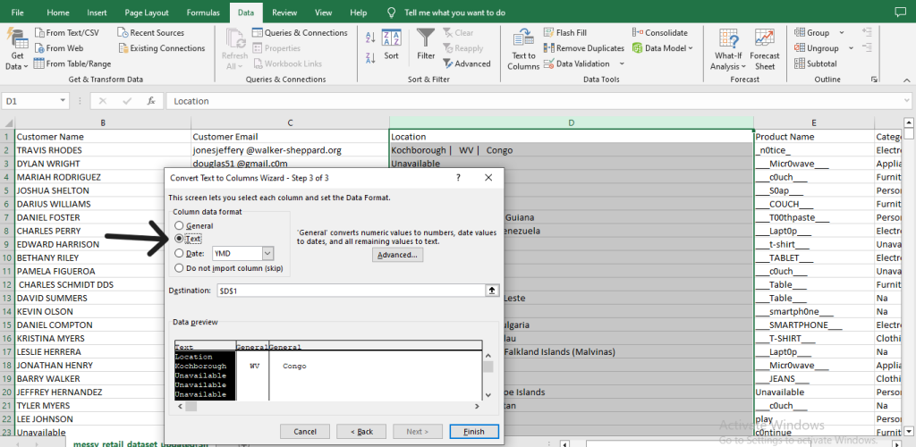
Excel “Convert Text to Columns Wizard 3 

7. All that’s left is to give the new columns an appropriate header. 

And with that you have successfully split a column using a character as a delimiter. 

Reversing Text Characters 

There may be instances where you might need to reverse the order of a text string, such as flipping names. 

Excel doesn’t have an in-bult function for reversing text string, but we can achieve this by using a combination of the TEXTJOIN, MIN, LEN and SEQUENCE functions. 

Before we proceed with reversing the text in the column, we need to ensure that we only reverse the entries that are actually written in reverse.

In our dataset, we recognize that not all names in the “Sales Representative” column are in reverse. Therefore, we must exclude those names that are already written correctly. 

One useful observation is that the reverse text tend to end with an uppercase letter (the last letter is capitalized), which would not be typical in properly written names.

We can use this as a condition to identify names which are in reverse. 

To filter and reverse only those names that are in reverse, we can use the following logic: 

IF(AND(CODE(RIGHT(J2,1))>=65, CODE(RIGHT(J2, 1))<=90), [Reverse Formula], J2).

This formula checks whether the last character is an uppercase letter (A-Z), using the CODE and RIGHT function. If the condition is true then it applies the reversal logic, otherwise, it leaves the text unchanged. 

1️⃣ RIGHT(J2,1) 

• It gets the last character of the text 

2️⃣ CODE(RIGHT(J2,1)) 

• The code function then returns the ASCII code of the last character 

• For example, A = 65, Z = 90, a = 97 etc. 

3. AND(CODE(RIGHT(J2,1))>=65, CODE(RIGHT(J2, 1))<=90) 

• Next, Excel checks if the ASCII code of the last character falls between 90 and 65, the ASCII range for uppercase letters.

4. IF(…….., [Reverse Formula], J2) 

• If the last character is an uppercase letter, it assumes the name is written in reverse and applies the reversal formula. 

• If not, it leaves the text by simply returning the original value in J2. 

When used in tandem with the text reversal formula =TEXTJOIN(“”, TRUE, MID(J2, SEQUENCE(LEN(J2),, LEN(J2), -1), 1)), it will reverse only the text that actually needs reversal. The text reversal formula works this way: 

1. LEN(J2) 

• This gives the length of the string in cell J2. 

• For example, if J2 is “skoorB hpesoJ”, then LEN(J2) would return 13. 

2. SEQUENCE(LEN(J2),, LEN(J2), -1) 

• Generates a list of positions from last to first. 

• If J2 is “skoorB hpesoJ”, then the formula returns 13, 12, 11, 10……1. 

3. MID(J2,….., 1) 

• This returns specific characters from the text, given a starting position and number of characters. 

• From our example, if J2 is “skoorB hpesoJ”, the formula pulls out: 13th character “J”, 12th character “o”, 11th character “s”, 10th character “e” all the way down to the 1st character “s” 

• This forms an array of reversed characters i.e. “J”, “o”, “s”, “e”, “p”, “h”, “ “, “B”, “r”, “o”, “o”, “k”, “s”. 

4. TEXTJOIN(“”, TRUE, ……) 

• This joins the resulting array of characters into one single string with no separator. 

• The “” means there should be no space between the characters, while the TRUE means that the formula should ignore any empty cells. 

• From our example, “J”, “o”, “s”, “e”, “p”, “h”, “ “, “B”, “r”, “o”, “o”, “k”, “s” becomes “Joseph Brooks”. 

So, joining all the formulas together to correctly reverse the text, we: 

1. Create a new column next to the desired column and give it the same name as the original column. 

2. In the second cell of the new column (column L), write the formula =IF(AND(CODE(RIGHT(J2, 1))>=65, CODE(RIGHT(J2, 1))<=90), TEXTJOIN("", TRUE, MID(J2, SEQUENCE(LEN(J2),, LEN(J2), -1), 1)), J2). This reverses the text string of in the “Sales Representative” that ends with an uppercase. 

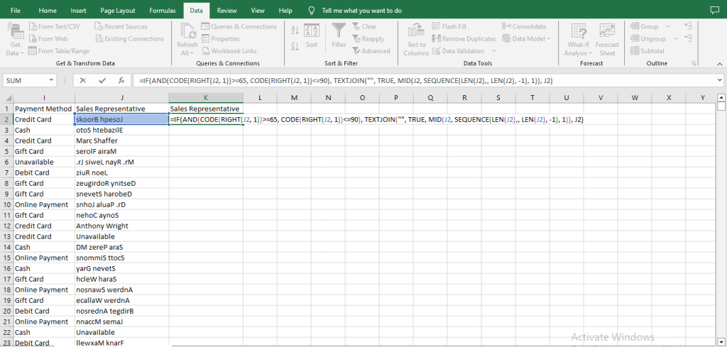
Text Reversal Formula 

3. Auto fill the remaining cells in the column. 

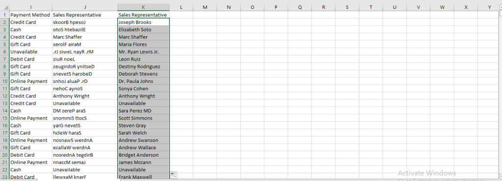
Names Reversed 

4. Copy the contents of the new “Sales Representative” column and past as values. 

This combination of functions, in this order, effectively flips the names that were originally written backwards. 

Although this method is very useful in reversing only the names that need to be reversed, it does have some limitations. 

A notable limitation involves names with suffixes such as “PhD”, “MD”, “III” etc. This suffix usually ends in uppercase letters, which means that our logic of checking if the last character of the text is an uppercase letter would end up wrongly flagging them as a reversed text.

As a result, names that are already written correctly, but contain these suffixes may be incorrectly reversed.

To handle this issue, after successfully reversing the names, filter the data to only display names that are not written in proper case.

Then review the filtered names for any that was wrongly reversed, before manually correcting any wrongly reversed name.

Since the filtered data contains only 247 rows, and only around 20 names were actually affected, this manual correction method is both practical and efficient. To do this, we: 

1. Create a new column (column L) next to our cleaned “Sales Representative” column. 

2. On the second cell of the new column (L2), write the formula  =EXACT(K2, PROPER(K2)). This formula checks if the reversed name is in proper case or not. It does this by: 

1. PROPER(K2) 

• This converts the text in the cell to a proper case. 

2. EXACT(K2, PROPER(K2)) 

• This checks if the original text is exactly the same as the proper case version. 

• If the text is in proper case, it returns TRUE 

• If the text is not in proper case, it returns FALSE 

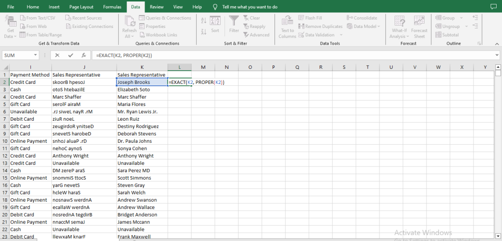
Checking for Proper Case Names 

3. Fill the rest of the column. 

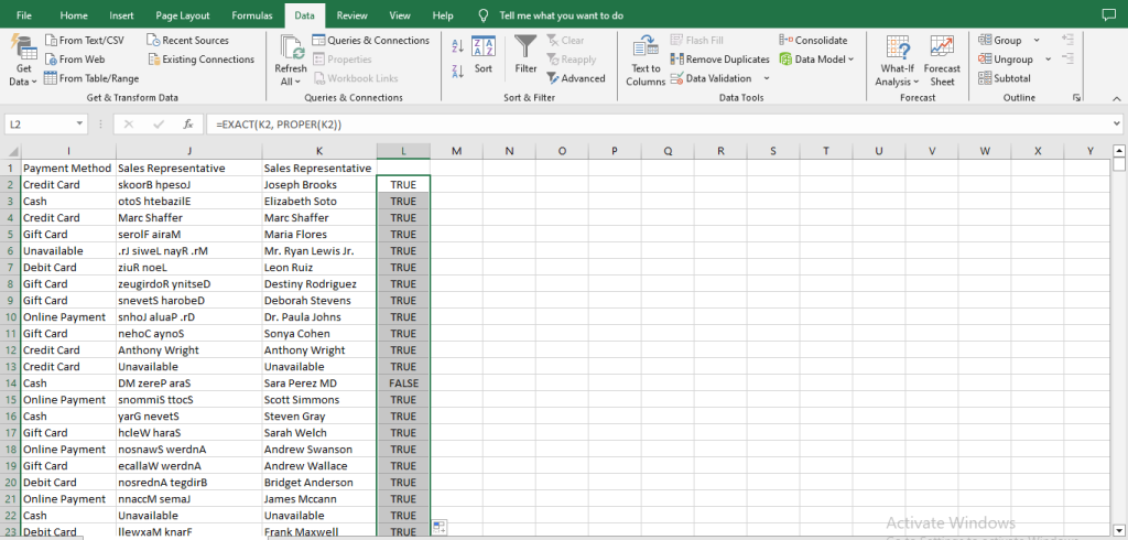
Filled Column L 

4. Go to Data on the menu bar, then select the Filter under Sort & Filter. 

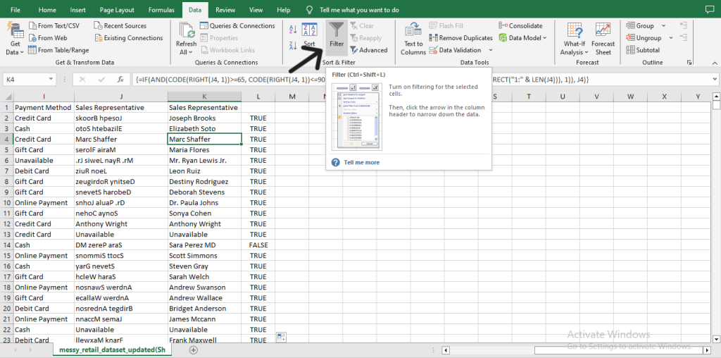
Selecting Filter Icon 

5. Hover your mouse to the funnel shaped icon on the righthand side of the column L header row and click on it. A drop-down menu will appear. 

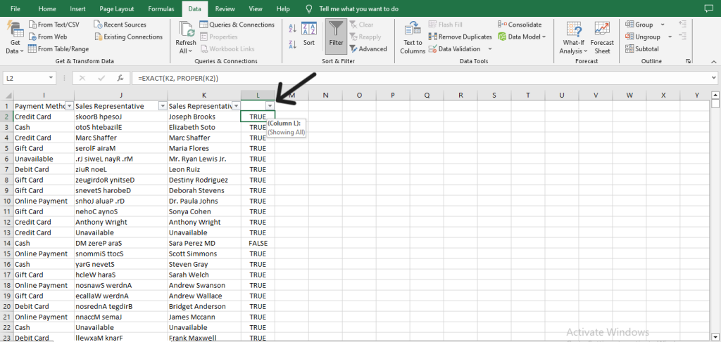
Filtering Column L 

6. From the drop-down menu that appears, make sure only FALSE is ticked, then click on Ok. This will filter out all the names that are in proper case and we’ll be left with the text that aren’t. 

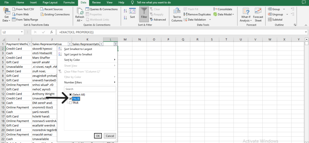
Filtering Only False Values on Column L 

7. Go through the entries on the reversed “Sales Representative” column (column K) and identify any name that were incorrectly reversed. To do this simply copy the correct version of the name from the original “Sales Representative” column (column J) and paste it into the corresponding cell in the reversed “Sales Representative” column (column K). 

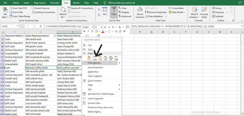
Pasting Values Only 

8. Removing the filter on column M; by clicking on the same icon you clicked to create the filter, then selecting Clear Filter From “(Column L)”. 

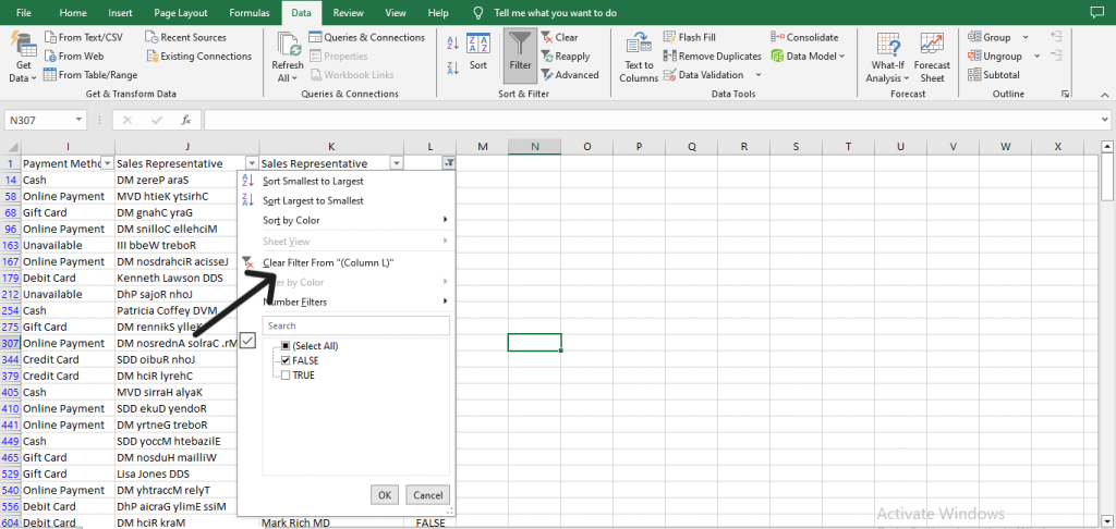
Clearing Column L Filter 

9. Hover back to Sort & Filter and click on Filter to completely remove the filter. 

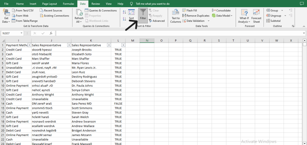
Removing Filter 

10. Delete the original “Sales Representative” column (column J), as well as column L. 

After that lengthy process, we have finally successfully reversed only the names that were incorrectly written. 

Common Pitfalls & Troubleshooting 

• If you don’t check the ‘My Data Has Headers’ box when removing duplicates, Excel might treat the first row as regular data—potentially removing important headers as duplicates. To avoid this, always double-check that the box is selected.

• When handling blank cells, forgetting to press Ctrl + Enter can result to only the active cell being filled rather than all the selected blank cells. So always remember to use Ctrl + Enter when filling multiple cells simultaneously. 

• Converting case to proper may alter acronyms or names that require specific casing (e.g. “SQL” might become “Sql”). So, after applying PROPER, manually convert any text that requires a different casing, or use conditional logic to handle such cases. 

• The text reversal formula relies on the SEQUENCE function, which is only available on Excel 365 or Excel 2021. Make sure your Excel is up to date to use this feature. 

Conclusion 

Cleaning data in excel is an essential skill for data analyst, as it ensures the accuracy, consistency and reliability of your analysis.

In this guide we’ve covered essential techniques like removing duplicates, handling blank cells, eliminating unwanted characters, trimming extra spaces, changing text cases, splitting delimited text and reversing text strings. 

By learning how to clean text data in Excel, you can transform messy data into a clean and organized dataset ready for analysis.

Clean data is the foundation of good analysis, and Excel’s tools make the process efficient and manageable, leading to better insights and decision making. 

If you’re also interested in cleaning the Date/Time data as well as the Numerical data, you can check out these very helpful guides on Cleaning Date/Time Data in Excel and Cleaning Numerical Data in Excel. 

To learn more about the Excel functions that were used in this guide as well as other powerful Excel functions, visit Microsoft’s official Excel function documentation.